A first step in random matrix theory

Preliminary remark: Over he past decade, the random matrix community provided plenty of relevant and interesting resources for the in-depth study of theoretical concepts. Some of these can be found in Terrence Tao's blog or in several books on the topic like A first course in random matrix theory. The aim of this page is to give someone with basic knowledge in mathematics and/or physics some first ideas of what random matrix theory is about and the fundamental tools used to describe them, without going into deep details and heavy formalism that you can easily find in many references. The introduction of these tools will also be useful for a further lesson introducing the use of statistical physics for understanding machine learning.

1. Random matrices and the Gaussian orthogonal ensemble

Simply put, a random matrix is a matrix whose elements are random variables. Random matrices are key objects naturally arising in several fields of science from physics, machine learning and chemistry to finance and ecology. In physics, it was introduced in the 1950s by Wigner who linked the statistics of the spacing between energy levels of atoms to the spacing between eigenvalues of a random matrix. Since then, random matrices appeared (and keep appearing) ubiquitously in diverse thematic of theoretical physics like quantum chromo-dynamics, spin-glasses, string theory, etc.

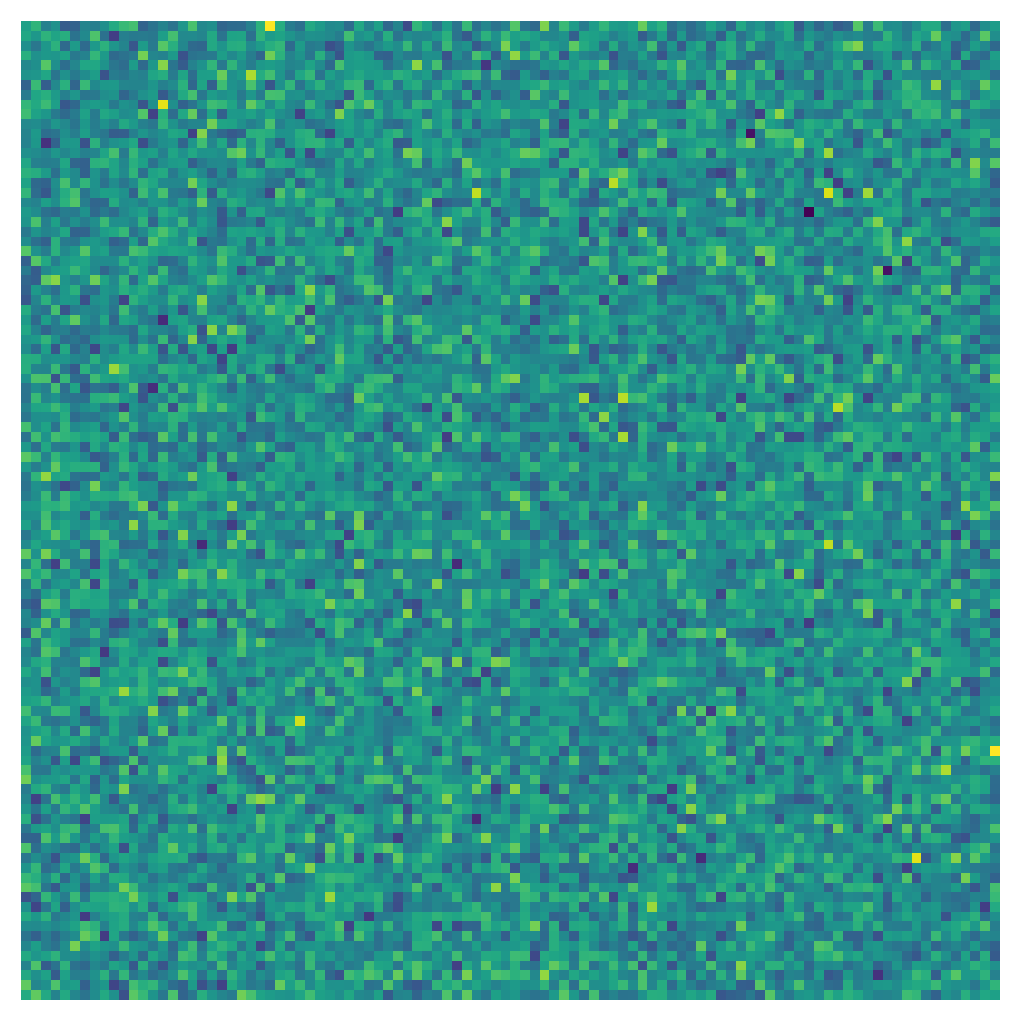
The type of objects we are interested in are hence square matrices $\boldsymbol{M} \in \mathbb{R}^{N \times N}$ where each element $m_{ij}$ is a random variable. An example of such a matrix is reproduced in the figure below where $N=100$ and $m_{ij} = m_{ji}$ are drawn from a centred Gaussian distribution of variance $1/N$, noted $\mathcal{N}(0, 1)$ with twice the variance on the diagonal, meaning that each pixel that you see is a realisation of a Gaussian variable. As can be intuited and appreciated visually, there is no particular pattern since each element is an independant realisation of all others.

Mathematically, we can write that $$ \boldsymbol{M} = \frac{\boldsymbol{J} + \boldsymbol{J}^\mathrm{T}}{\sqrt{2N}}, $$

where we added $N$ to normalize the matrix and $\boldsymbol{J}$ is a random matrix with $j_{ij} \sim \mathcal{N}(0,1)$. Such matrices are called Gaussian Wigner matrices and belong to the Gaussian orthogonal ensemble (GOE) because their symmetry makes them invariant under orthogonal transformations.

Why is that important?

Many results of random matrix theory are derived by relying on one of the following assumption: i) the entries of the matrix are independant; ii) the matrix is invariant under some transformations (orthogonal in real case or unitary in complex case). These are, grossly speaking, the two cases in which the existing mathematical tools allow to study the random matrices in details from an analytical perspective. The type of matrix we have built just before, with Gaussian independant entries, is a very particular case since it belongs to the two families described here: it is a matrix with independant entries but is also invariant under orthogonal transformations. In fact, the GOE is the only ensemble fulfilling simultaneously these two conditions.

While independance of the entries is straightforward to see, the invariance under orthogonal transformation can be deduced when writing the probability measure associated with the ensemble as

$$ \begin{align} p(M) &= \exp\left(\frac{-N\sum_{i \neq j}^N m_{ij}^2}{4} - \frac{N\sum_{i=1}^N m_{ii}^2}{4} \right) \\\
&= \exp\left(\frac{-N\sum_{i, j = 1}^N m_{ij}^2}{4} \right) \\\
&= \exp\left(\frac{-N}{4} \mathrm{Tr} \boldsymbol{M}^2 \right), \end{align} $$

where $\mathrm{Tr} \boldsymbol{M}$ designates the trace of the matrix $M$ (i.e. the sum of its diagonal elements). We hence see that if we take $\boldsymbol{M}^\prime = \boldsymbol{O} \boldsymbol{M} \boldsymbol{O}^{\mathrm{T}}$ with $\boldsymbol{O}$ an orthogonal matrix, the measure remains unchanged.

The first thing one wants to have a look at when dealing with a matrix are its eigenvalues that are linked with many properties of the system the matrix represents such as the stability of a dynamical system or the energy levels of vibrating atoms. As a reminder, the eigenvalues $\lambda_i$ of a matrix are defined as the factors multiplying the directions that remain unchanged by application of the matrix $\boldsymbol{M}$ (the so-called eigenvectors $\boldsymbol{v}_{i}$),

$$ \boldsymbol{M} \boldsymbol{v}_i = \lambda_i \boldsymbol{v}_i. $$

For our matrix $\boldsymbol{M}$, we hence have $N$ eigenvalues that we order ascendingly as $\lambda_1 \leq \lambda_2 \leq \cdots \leq \lambda_N$. A generic question that one may ask is ''How are the eigenvalues of the random matrix at hand distributed?''. This question is actually at the heart of random matrix theory and mathematicians have developped several tools allowing to answer it. Our goal for the next few sections is to introduce these tools, use it to compute analytically the distribution of eigenvalues of our matrix $\boldsymbol{M}$ above and compare it with numerical simulations.

2. Stieltjes transform and eigenvalue distribution

The Stieltjes transform is a crucial element of random matrix theory that provides information on the moments of the random matrix and the density of eigenvalues. It is defined as

$$ g_{\boldsymbol{M}}(z) = \frac{1}{N} \sum_{i=1}^N \frac{1}{z - \lambda_i}, \label{eq:Stieltjes_def}\tag{1} $$

for $z$ in the complexe plane excluding the eigenvalues $\lambda_i$. The Stieltjes transform can be written matricially as the normalised trace of some matrix $\boldsymbol{G}_{\boldsymbol{M}} = (z\boldsymbol{I} - M)^{-1}$ called the resolvent of $\boldsymbol{M}$,

$$ g_{\boldsymbol{M}} = \frac{1}{N} \mathrm{Tr} \, {\boldsymbol{G}_\boldsymbol{M}}. $$

The two formulations are equivalent and the knowledge of $\boldsymbol{G}_{\boldsymbol{M}}$ implies the one of the Stieltjes transform (note however that the reciprocal is not true).

With this definition, we directly see that the eigenvalues of $\boldsymbol{M}$ are linked in a very particular way to the Stieltjes transform since they cancel out the denominator and are hence excluded from the interval of definition of $g_{\boldsymbol{M}}$. Mathematicians formulated this idea through the Sokhotski–Plemelj formula that links the density of eigenvalues $\rho(\lambda)$ and the Stieltjes transform as

$$ \rho(\lambda) = \frac{1}{\pi} \operatorname*{lim}_{\epsilon \rightarrow 0^+} \mathrm{Im} \, \mathcal{g}(\lambda - i\epsilon). \label{eq:Stieltjes_inverse}\tag{2} $$

This formula may look scary at first sight but let's decompose it. It says that the density of eigenvalues can be obtained by evaluating the Stieltjes transform at a precise complex number that is $\lambda - i \epsilon$ with a very small $\epsilon$. This makes sense because we have seen before that the Stieltjes transform is not defined at eigenvalues $\lambda$ but taking it slightly away along the complex axis is authorized. Why not along the real axis you may ask? Well, if we consider the eigenvalue density as a continuum, then "slightly away" from $\lambda_i$ on the real axis is $\lambda_j$, another eigenvalue at which we cannot evaluate the Stieltjes transform. However, since in our case the matrix is symetric, all the eigenvalues are real and along the complex axis, we are not bothered by other eigenvalues and the Stieltjes transform is well defined. Let us now have a look at the imaginary part of this quantity

$$ \mathrm{Im} , \mathcal{g}(\lambda - i\epsilon) = \frac{1}{N} \sum_k \frac{\epsilon}{\left(\lambda - \lambda_k\right)^2 + \epsilon^2}, $$

and taking the $\epsilon \rightarrow 0^+$ limit leads to $$ \begin{align} \operatorname*{lim}_{\epsilon \rightarrow 0^+} \mathrm{Im} \, \mathcal{g}(\lambda - i\epsilon) &= \frac{\pi}{N} \sum_{k=1}^N \delta(\lambda - \lambda_k), \\\
&= \pi \rho(\lambda) \end{align} $$

where $\delta(x)$ denotes the Dirac delta distribution and where we used the alternative definition $\delta(x) = \frac{1}{\pi} \operatorname*{lim}_{\epsilon \rightarrow 0^+} \frac{\epsilon}{x^2 + \epsilon^2}$.

3. Eigenvalue distribution of the GOE: the Wigner semi-circle law

Equipped with the Stieltjes transform and its inverse transform, we are now interested in mathematically describing the eigenvalue distribution of the GOE. We know from the previous section that the first thing we need to compute is the Stieltjes transform of $\boldsymbol{M}$. It turns out that the expected value of $g_{\boldsymbol{M}}$, denoted $g$, satisfies a pretty simple equation in this case which is

$$ g - zg + 1 = 0, \label{eq:resolvent_eq_GOE}\tag{3} $$ or equivalently $$ g(z) = \frac{z \pm \sqrt{z^2 - 4}}{2}. $$

How to derive this expression?

There are different ways to compute the resolvent matrix $\boldsymbol{G}$ coming from physics (in which context it is called a Green function) or mathematics to then derive the Stieltjes transform which corresponds to its trace. We expose here a brute-force computation relying on some results from mathematics and we will see in a further post how to come up with the same result based on tools coming from theoretical physics.

We first make use of the rotational invariance of the problem as we saw earlier and can hence compute the element $g_{11}$ of the resolvent and then use the fact that $g_{\boldsymbol{M}} = \frac{1}{N} g_{11}$. To do so, we decompose the input matrix $\boldsymbol{A} = z\boldsymbol{I} - \boldsymbol{M}$ into four blocks

$$ \boldsymbol{A} = \begin{pmatrix} a_{11} & \boldsymbol{A}_{12} \\\
\boldsymbol{A}_{21} & \boldsymbol{A}_{22} \end{pmatrix}, $$

where $a_11$ is the scalar entry $(1,1)$ of the matrix, $\boldsymbol{A}_{12}$ and $\boldsymbol{A}_{21}$ are vectors excluding the first element and $\boldsymbol{A}_{22}$ is a $(N-1)\times (N-1)$ matrix.

Inspecting the elements of this matrix, we first remark that $a_{11} = z - m_{11}$ and $\boldsymbol{A}_{12} = -\boldsymbol{M}_{12}$ since $z$ is only acting on the diagonal. The last remark is that $\boldsymbol{A}_{22}$ is in fact the inverse resolvent matrix of a Wigner matrix of size $N-1$. From this decomposition, we can use the Schur complement formula, to compute the first element of the inverse of $\boldsymbol{A}$, i.e. $g_{11}$. This goes as

$$ g_{11} = \frac{1}{a_{11} - \boldsymbol{A}_{12} \boldsymbol{A}_{22}^{-1} \boldsymbol{A}_{21}} $$

Now, we need to take the expectation of this equation over the random variables $m_{ij}$.

Let us do it term by term:

1. The first term $g_{11}$ is simply the expectation of one term of the diagonal of the resolvent. By rotation invariance, it is given by

   $$ \mathbb{E}(g_{11}) = \frac{1}{N} \mathbb{E}(\mathrm{Tr} \,\boldsymbol{G}) = g. $$

2. For the denominator, we first have

   $$ \mathbb{E}(a_{11}) = \mathbb{E}(z - m_{11}) = z, $$

   since $m_{11}$ is a centred Gaussian random variable.

3. Finally, let us decompose the last term as

   $$ \sum_{i,j=1}^N \mathbb{E}( a_{1i} (\boldsymbol{A}_{22}^{-1})_{ij} a_{j1} ), $$

   where we simply re-wrote the product of matrices as a sum.

   Since the elements of the first row and column are independant from other elements in the Wigner ensemble, we obtain

   $$ \begin{align} \mathbb{E}( a_{1i} (\boldsymbol{A}_{22}^{-1})_{ij} \boldsymbol{a}_{j1}) &= \mathbb{E}(a_{1i} a_{j1}) \, \mathbb{E}((\boldsymbol{A}_{22}^{-1})_{ij}), \\\
   &= \mathbb{E}(x_{1i} x_{j1}) \, \mathbb{E}((\boldsymbol{A}_{22}^{-1})_{ij}), \\\
   &= \frac{1}{N} \delta_{ij} \, \mathbb{E}((\boldsymbol{A}_{22}^{-1})_{ij}). \end{align} $$

   This gives us for the full sum $\mathbb{E}(\boldsymbol{A}_{12} \boldsymbol{A}_{22}^{-1} \boldsymbol{A}_{21}) = \frac{1}{N} \mathbb{E}(\boldsymbol{A}_{22}^{-1}).$

   From our previous observation, we know however that $\boldsymbol{A}_{22}$ is a Wigner matrix itself of size $(N-1) \times (N-1)$. This means that we have

   $$ \frac{1}{N-1} \mathbb{E}(\boldsymbol{A}_{22}^{-1}) = g. $$

   What we have is however not a denominator of $N-1$ but $N$. To pursue the calculation, we set put ourselves in the context of high-dimension limit where $N \approx N - 1$ when $N \gg 1$.

   Putting it all together from the Schur complement formula, we obtain

   $$ g = \frac{1}{z - g}, $$

   which gives back Eq. (\ref{eq:resolvent_eq_GOE}).

We remark that this last equation provides us with two possible answers depending on the sign in front of the square root. One way of choosing the correct sign is to remember the definition of the Stieltjes transform in Eq. (\ref{eq:Stieltjes_def}). We see that for a very large $z$, $g(z)$ behaves as $1/z$. The only way for us of getting this behaviour is to take the minus sign hence leading to

$$ g(z) = \frac{z - \sqrt{z^2 - 4}}{2}. $$

More details about the sign

We have that

$$ g(z) = \frac{z \pm \sqrt{z^2 - 4}}{2} $$

and want to choose the sign giving the correct asymptotic behaviour when $z$ is large. To do so, we re-write the expression in such a way we can perform a Taylor expansion of the square root, i.e. something of the form $\sqrt{1 - \epsilon}$ with $\epsilon$ a term going to $0$. This can be achieved by factorizing the $z^2$ in the square root giving

$$ g(z) = \frac{z \pm z\sqrt{1 - 4/z^2}}{2}. $$

From there, a Taylor expansion at first order reads

$$ \begin{align} g(z) &\approx \frac{z}{2} \pm \frac{z}{2}(1-\frac{2}{z^2}), \\\
&\approx \frac{z}{2} \pm \frac{z}{2} \mp \frac{1}{z}. \end{align} $$

Consequently, if we choose the positive sign, we end up with a $z$ behaviour while the negative one cancels the $z$ to give the $1/z$ that we expect from the Stieltjes transform definition.

After these efforts, let us pause a moment to think about what we have done and where we stand. So far, we computed the expected Stieltjes transform of matrices from the GOE and obtained a closed-form formula for $g(z)$. What we wanted to compute is the distribution of eigenvalues that is linked with the Stieltjes transform by the Sokhotski–Plemelj formula from Eq. (\ref{eq:Stieltjes_inverse}). It is given by

$$ \begin{align} \rho(\lambda) &= \frac{1}{\pi} \operatorname*{lim}_{\epsilon \rightarrow 0^+} \mathrm{Im} \, \mathcal{g}(\lambda - i\epsilon), \\\
&= \frac{1}{\pi} \operatorname*{lim}_{\epsilon \rightarrow 0^+} \mathrm{Im} \, \frac{-\lambda - i\epsilon + \sqrt{\lambda^2 - \epsilon^2 - 4 +2i\lambda \epsilon} }{2}, \\\
&= \begin{cases} 0, & \mathrm{if }|\lambda| > 2, \\\
\frac{1}{2\pi} \sqrt{4-\lambda^2}, & \mathrm{if }|\lambda| < 2, \end{cases} \end{align} $$

where for the last equality, we used the principal square root definition of complex numbers.

Principal square what?

The equality we used is

$$ \sqrt{a + ib} = p+iq, $$

where

$$ \begin{align} p &= \frac{1}{\sqrt{2}} \sqrt{\sqrt{a^2 + b^2} + a}, \\\
q &= \frac{\mathrm{sign}(b)}{\sqrt{2}} \sqrt{\sqrt{a^2 + b^2} - a}. \end{align} $$

From this, we can re-write the square root of the distribution and compute easily the limit to obtain the Wigner semi-circle law.

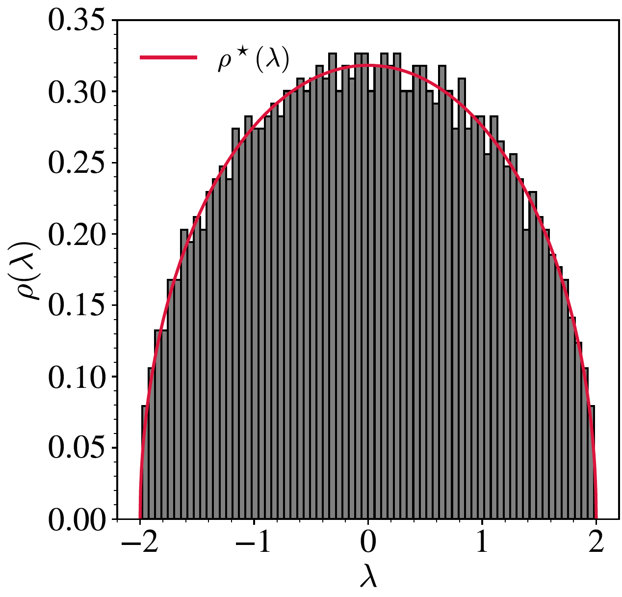
This is finally done! We derived together the famous Wigner semi-circle law. Our derivation should be valid in the large dimension $N$ limit and provide the exact asymptotic distribution of eigenvalues of individual matrices from the GOE. Let us see how this theoretical prediction is comparing to a numerical simulation. The comparison is shown below where the red line is our theoretical prediction and the histogram is the density estimation of a single matrix with $N=2000$. We see a pretty good agreement between the two, even if $N$ is not properly infinite in the simulation!

4. Going further

• In this post, we conducted the computation of the exact asymptotic distribution of eigenvalues but a large part of research activities in random matrix theory also focused on the fluctuations of the eigenvalues and "how plausible" it is for an eigenvalue (especially those at the border) to fluctuate at finite values of $N$. In the case of GOE we studied, these fluctuations of extreme eigenvalues at the border are known to be Tracy-Widom distributed with a scaling factor of $N^{-2/3}$.

• In reality, random matrix theory can provide us with much more information about this problem, such as what happens when we add a small rank perturbation to a random matrix. In this case, we can compute the precise overlap we can expect to have between the signal $\boldsymbol{v}$ and its estimation by the largest eigenvalue, but also the position of the outlier eigenvalue and the value of the signal-to-noise ratio at which the signal can be found or not. All these will have a dedicated post in a near future!

• One can also extend all these analyses to other random matrix ensemble, such as the set of covariance matrices of the form

$$ \boldsymbol{M} = \frac{1}{T} \sum_{i=1}^T \boldsymbol{x} \boldsymbol{x}^\mathrm{T}, $$

where the same kind of results for the eigenvalue distribution can be obtained and leads to what is called the Marcenko-Pastur distribution which is hence the equivalent of the Wigner semi-circle law for this matrix ensemble.