Mixture models and Expectation-Maximisation algorithm
Context
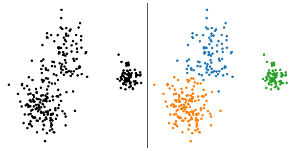
Clustering is a one of the most ancient unsupervised tasks of ML aiming at identifying a partition of a given dataset into multiple groups called "clusters". The plot below illustrates this objective in a 2D case where the aim is to go from the left panel to the right one, by attributing a class to each input datapoint.
The common ground to many methods that have been proposed these past decades is that they all embed, in some ways, a measure of the "similarity" between datapoints living inside the same cluster. The simplest way of thinking this is a measure based on the Euclidean distance leading to representations in which "close" datapoints more likely fall into the same cluster while distant ones should reside in different clusters. The prototypical method to partition a $D$-dimensional dataset into $K$ clusters is the K-means algorithm proposed by Macqueen in 1967. We can write the K-means goal as the optimisation problem aiming at finding the set of $K$ points (hereafter called centres) minimising the sum of squared distances between datapoints and cluster centres. We end up in a setting seeking to find the set of points $\left( \boldsymbol{\mu}_1, \ldots, \boldsymbol{\mu}_K \right)$ minimising
$$ \sum_{i=1}^N \operatorname*{min}_{k \in \lbrace 1, \ldots, K \rbrace } \lVert \boldsymbol{x}_i - \boldsymbol{\mu}_k \rVert^2_2. $$
The K-means algorithm solves this optimisation problem in a simple way. Starting from a set of initial positions ${\mu}^{(0)}$, it assigns to each datapoint $\boldsymbol{x}_i$ the closest (in the sense of the Euclidean distance) centroid among $\boldsymbol{\mu}$, noted ${\mu}({x}_i)$, and moves ${\mu}_k$ accordingly to the average of all datapoints projecting on it, namely $\boldsymbol{\mu}_k^{(t+1)} = \mathbb{E}(\boldsymbol{x}_i | \boldsymbol{\mu}({x}_i) = \boldsymbol{\mu}_k^{(t)})$. As we can see, this formulation assigns a single centroid to a datapoint without any level of uncertainty, making it a "hard" version of clustering. In case of overlapping clusters, such as the two on the left of the first Figure, it is however natural to think that datapoints living at the border could be either in the blue or the orange cluster. Also, because the association energy appearing in the above equation is based on the Euclidean distance, it tends to generate spherical groups. These restrictions of the K-means algorithm later led to the Gaussian mixture model formulation of the clustering. This latter introduces a fuzziness by assigning a probability to each datapoint of being generated by one the $K$ clusters but also extends the definition to anisotropic clusters of various densities. Let us see how it works!
Mixture models
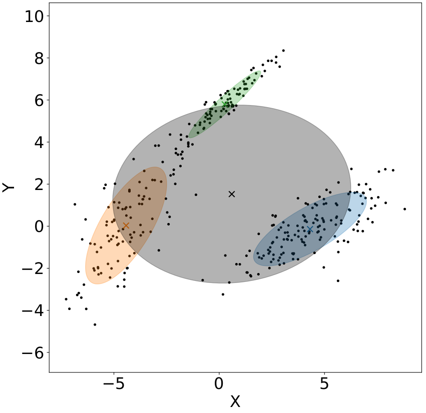
Real-life data often come as drawn from probability distributions with complex shapes and multiple modes that cannot be satisfactorily described by a single well-known probability distribution. Mixture models propose to model this complexity by using a linear combination of $K$ known laws. The Figure below illustrates this need on a multi-modal 2D distribution of points. Although easy to study, a single Gaussian component (the grey ellipse) do not explain fairly well the non-Gaussian dataset while a linear combination of three Gaussian (the set of coloured ellipses) is leading to a better representation.
Mathematically, a mixture distribution is the linear combination of $K$ probability distributions individually denoted $ f_k(\boldsymbol{x},\boldsymbol{\theta}_k) $ with parameters $ \boldsymbol{\theta}_k $. The probability of a datapoint $ \boldsymbol{x} $ being generated by the model is hence
$$ p(\boldsymbol{x} | \boldsymbol{\Theta}) = \sum_{k=1}^K \pi_k f_k(\boldsymbol{x}, \boldsymbol{\theta}_k), $$
with $\boldsymbol{\Theta} = \lbrace \pi_1, \ldots, \pi_K, \boldsymbol{\theta}_1, \ldots, \boldsymbol{\theta}_K \rbrace $ the set of model parameters where $ \pi_k $ is the mixing coefficient (also called amplitude) of component $k$. Note that, given the properties of probability distributions, amplitudes are normalised and positive by definition, namely $ \sum_{k=1}^K \pi_k = 1$ and $\forall k \in \lbrace 1, \ldots, K \rbrace, \pi_k \geq 0 $.
This idea of combination of known laws, despite its conceptual simplicity, can lead to accurate representations of highly complex density distributions! This is in particular why mixture distributions are nowadays at the basis of many mathematical tools used in machine learning like kernel density estimation, clustering or mixture density networks.
A particular class of mixture model is the Gaussian case, where $\forall k \in \lbrace 1, \ldots, K \rbrace, f_k(\boldsymbol{x}, \boldsymbol{\theta}_k) = \mathcal{N}(\boldsymbol{x}, \boldsymbol{\theta}_k)$, with
$$ \mathcal{N}(\boldsymbol{x}, \boldsymbol{\theta}_k) = \frac{\exp{ -\frac{1}{2} \left(\boldsymbol{x} - \boldsymbol{\mu}_k\right)^\mathrm{T} \boldsymbol{\Sigma}_k^{-1} \left(\boldsymbol{x} - \boldsymbol{\mu}_k\right)}}{(2\pi)^{D/2} \lvert \boldsymbol{\Sigma}_k \rvert^{1/2}}, $$
the Gaussian probability distribution with parameter $\boldsymbol{\theta}_k = \lbrace \boldsymbol{\mu}_k, \boldsymbol{\Sigma}_k \rbrace$, respectively corresponding to the average of the $k^\mathrm{th}$ Gaussian component and its covariance matrix.
Expectation-Maximisation
For now, we have modelled our datasets with a linear combination of $K$ laws. We now need to estimate to optimal set of parameters $ \boldsymbol{\Theta} $ that fit a given dataset $ \boldsymbol{X} = \lbrace \boldsymbol{x}_{i} \rbrace$.
As usually done in statistics, we can do that by maximising the likelihood of the model. Intuitively, the likelihood encode the information of how probable it is that our observed dataset was generated by the model. Mathematically, it is written $p(\boldsymbol{X} | \boldsymbol{\Theta}) $ and is often expressed in $\log$ for convenience. Assuming independence of the datapoints and a mixture model, we can simply write the log-likelihood as the product of all individual probabilities, which in $\log$ gives:
$$ \log p( \boldsymbol{X} | \boldsymbol{\Theta}) = \sum_{i=1}^N \log \left( \sum_{k=1}^K \pi_k f_k(\boldsymbol{x}_i, \boldsymbol{\theta}_k) \right). $$
Unfortunately, this log-likelihood is not analytically tractable because of the summation appearing inside the log function!
One clever way to circumvent this was proposed by Dempster in 1977 and it is called the Expectation-Maximisation. It first reformulates the mixture model in terms of _latent variables_, by simply introducing a set of random variables $\boldsymbol{Z} = \lbrace z_i \rbrace_{i=1}^N $ with $ z_i \in \lbrace 1, \ldots, K \rbrace$. In fact, $\boldsymbol{Z}$ represents the partition of the dataset and $z_i$ denotes by which of the $K$ component the datapoint $\boldsymbol{x}_i$ has been generated from. The latent variables $\boldsymbol{Z}$ can simply be seen as the answer we are looking for in the clustering problem! Now imagine that we have access to them, we can write the new log-likelihood,
$$ \log p(\boldsymbol{X}, \boldsymbol{Z} | \boldsymbol{\Theta}) = \sum_{i=1}^N \log \left(\pi_{z_i} f(\boldsymbol{x}_i, \boldsymbol{\theta}_{z_i}) \right). $$
This new log-likelihood $ \log p(\boldsymbol{X}, \boldsymbol{Z} | \boldsymbol{\Theta}) $ is often referred to as the "completed log-likelihood" of the model in the sense that the joint knowledge of datapoints $\boldsymbol{X}$ and latent variables $\boldsymbol{Z}$ is the "completed dataset". The idea behind EM is that the log-likelihood of $\lbrace \boldsymbol{X}, \boldsymbol{Z} \rbrace $ is easier to maximise than the one of our initial model. Simply said: if we knew the vector $\boldsymbol{Z}$, we could easily maximise the completed likelihood and find parameters $\boldsymbol{\Theta}$ of the model by simple derivations. Unfortunately, $\boldsymbol{Z}$ is not know! These are why we call them "latent", "hidden" or sometimes "unobserved" variables. We hence need to estimate them, in addition to $\boldsymbol{\Theta}$.
It might seem strange that I'm stating that the task is now easier since we now need to estimate two quantities: $\boldsymbol{\Theta}$ AND $\boldsymbol{Z}$ instead of just $\boldsymbol{\Theta}$ in the first place... But it is! When knowing $\boldsymbol{\Theta}$, estimate $\boldsymbol{Z}$ is easy, and when knowning this latter, estimating $\boldsymbol{\Theta}$ is easy! This is the key idea of the Expectation-Maximisation algorithm.
EM hence provides a procedure with two alternating steps to iteratively estimate both quantities. Let's dive into the mathematics of it. First, we can relate the two log-likelihood: the initial one $\log p(\boldsymbol{X} | \boldsymbol{\Theta})$ and the completed one $\log p(\boldsymbol{X}, \boldsymbol{Z} | \boldsymbol{\Theta})$. In fact, for any distribution over the latent variables $q(\boldsymbol{Z})$, we can derive the relation
$$ L(q, \boldsymbol{\Theta}) = - D_\mathrm{KL}(q, p(\boldsymbol{Z} | \boldsymbol{X}, \boldsymbol{\Theta})) + \log p(\boldsymbol{X} | \boldsymbol{\Theta}), $$
where $D_\mathrm{KL}(q, p) = \sum q \log q/p \geq 0$ is the Kullback-Leibler divergence and $L = \sum_{\boldsymbol{Z}} q(\boldsymbol{Z}) \log \left[ \frac{p(\boldsymbol{X}, \boldsymbol{Z} | \boldsymbol{\Theta})}{q(\boldsymbol{Z})} \right]$.
Want more information about the derivation of this equation?
Using Jensen's inequality, stating that, for any random variable $X$ and convex function $f$, $f(\mathbb{E} \lbrace X \rbrace) \leq \mathbb{E} \lbrace f(X) \rbrace$ and the concavity of the logarithm function, we can write the log-likelihood, for any normalised distribution $q(\boldsymbol{Z})$ over the latent variables, as
$$ \log p(\boldsymbol{X} | \boldsymbol{\Theta}) \geq L(q, \boldsymbol{\Theta}) = \sum_{\boldsymbol{Z}} q(\boldsymbol{Z}) \log \left[ \frac{p(\boldsymbol{X}, \boldsymbol{Z} | \boldsymbol{\Theta})}{q(\boldsymbol{Z})} \right]. $$
Hence, the log-likelihood of the model is bounded below by $L(q, \boldsymbol{\Theta})$. If easier to handle, maximising this quantity could help maximising $\log p(\boldsymbol{X} | \boldsymbol{\Theta})$. We can re-write this lower-bound, using the normalisation of $q(\boldsymbol{Z})$ and the decomposition $p(\boldsymbol{X}, \boldsymbol{Z} | \boldsymbol{\Theta}) = p(\boldsymbol{Z} | \boldsymbol{X}, \boldsymbol{\Theta}) p(\boldsymbol{X} | \boldsymbol{\Theta})$, which leads to the expression given above.
Because of the positivity of the Kullback-Leibler divergence, we see that $L(q, \boldsymbol{\Theta})$ is a lower-bound of the log-likelihood with $\log p(\boldsymbol{X} | \boldsymbol{\Theta}) \geq L(q, \boldsymbol{\Theta})$. So, maxisiming the lower-bound $L$ should increase the log-likelihood. As a first step, we can estimate the distribution $q(\boldsymbol{Z}$ of the latent variable that maximises the lower-bound. This is easy since the log-likelihood is independant from $\boldsymbol{Z}$ and the $D_\mathrm{KL}$ is positive! So we use the current values of the parameters $\boldsymbol{\Theta}^{(t)}$ and set
$$ \hat{q}(\boldsymbol{Z}) = p(\boldsymbol{Z} | \boldsymbol{X}, \boldsymbol{\Theta}^{(t)}). $$
This step is called the E-step as a reference to "Expectation" because the lower-bound can be written in terms of the Expectation of the completed log-likelihood over the distribution of latent variables.
From these estimate of latent variables, we can now maximises the lower-bound, or equivalently the log-likelihood since the Kullback-Leibler now cancels out. We consequently need to compute
$$ \boldsymbol{\Theta}^{(t+1)} = \operatorname*{argmax}_{\boldsymbol{\Theta}} L(\hat{q}, \boldsymbol{\Theta}), $$
This step is the M-step, standing for "Maximisation" because we need to maximise the lower-bound over the parameters of the model.
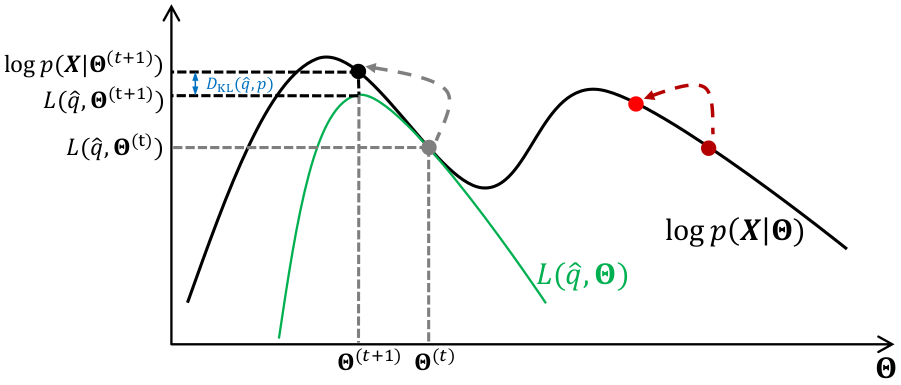
The full EM algorithm, by alternating between E and M steps, iteratively maximises the log-likelihood of the model through the double maximisation of a lower-bound, first over the distribution of latent variables and then over the parameters of the model, $\boldsymbol{\Theta}$. As shown in the Figure below, starting from a random initialisation (either the grey or dark red point), we iteratively climb the log-likelihood by using a simpler function to maximise, the lower-bound $L(\boldsymbol{q}, \boldsymbol{\Theta})$.
Application to Gaussian mixture models
We have seen the theoretical context of the Expectation-Maximisation algorithm for general mixtures. How can we use it in practice if we model our dataset with the Gaussian Mixture Model (GMM)?
Well, in this scenario, we can derive, in the E-step, the probability of the latent variables given the observed data and the current parameters of the model. This is what we call _responsibilities_ and we will note them $p_{ik} = p(z_i = k | \boldsymbol{x}_i, \boldsymbol{\Theta}^{(t)})$. They represent the probability of a datapoint $i$ being generated by the $k$th component of the model. Using Bayes' theorem,
$$ p_{ik} = \frac{\pi_k \mathcal{N}(\boldsymbol{x}_i, \boldsymbol{\theta}_k^{(t)})}{\sum_{j=1}^K \pi_j \mathcal{N}(\boldsymbol{x}_i, \boldsymbol{\theta}_j^{(t)})}. $$
Bayes theorem and the derivation
Bayes' theorem allows to express the probability of an event given some prior knowledge. In our context, we can write
$$ p(z_i = k | \boldsymbol{x}_i, \boldsymbol{\Theta}^{(t)}) = \frac{p( \boldsymbol{x}_i | z_i = k, \boldsymbol{\Theta}^{(t)} ) p(z_i = k | \boldsymbol{\Theta}^{(t)}) }{ p(\boldsymbol{x}_i | \boldsymbol{\Theta}^{(t)}) }. $$
The left term in the numerator is the probability of observing $\boldsymbol{x}_i$ knowing that it belongs to the cluster $k$ and the parameters of the model. The right one is the probability of $\boldsymbol{x}_i $ being in the cluster $k$ given parameters of the model. Finally, the denominator is the probability of observing $\boldsymbol{x}_i $ given parameters of the model and independantly of any belonging to Gaussian clusters.
This estimation of $p_{ik}$ is then used in the M-step to evaluate the maximum of the lower-bound
$$ L(q, \boldsymbol{\Theta}) = \sum_{i=1}^N \sum_{k=1}^K p_{ik} \log \left[ \pi_k \mathcal{N}(\boldsymbol{x}_i, \boldsymbol{\theta}_k) \right] + \mathrm{cst}. $$
Parameters of the model can be obtained by maximising this quantity over $\boldsymbol{\Theta}$. In the case of a GMM, the M-step consists then in solving
$$ \operatorname*{argmax}_{\boldsymbol{\Theta}} \sum_{i=1}^N \sum_{k=1}^K p_{ik} \left[ \log \pi_k - \frac{1}{2} \log \boldsymbol{\Sigma}_k - \frac{1}{2} \left(\boldsymbol{x}_i - \boldsymbol{\mu}_k \right)^\mathrm{T} \boldsymbol{\Sigma}_k \left(\boldsymbol{x}_i - \boldsymbol{\mu}_k \right) \right], $$
This equation is very similar to the one from the very first equation of the lesson, the one optimised by the K-means algorithm! However, in the K-means one, a datapoint is associated to a unique cluster while the GMM method not only includes a parameter for the shape of the cluster through the covariance matrices but also quantifies the probability of a datapoint to be represented by a given cluster $k$ through the responsibility $ p_{ik} $.
It is hence possible to derive an update equation for each parameter of $\boldsymbol{\Theta}^{(t+1)}$ as
$$ \pi_k^{(t+1)} = \displaystyle \frac{1}{N} \sum_{i=1}^N p_{ik}, $$ $$ \boldsymbol{\mu}_k^{(t+1)} = \frac{\sum_{i=1}^N \boldsymbol{x}_i p_{ik}}{\sum_{i=1}^N p_{ik}}, $$ $$ \boldsymbol{\Sigma}_k^{(t+1)} = \displaystyle \frac{\sum_{i=1}^N p_{ik} (\boldsymbol{x}_i - \boldsymbol{\mu}_k) (\boldsymbol{x}_i - \boldsymbol{\mu}_k)^\mathrm{T}}{\sum_{i=1}^N p_{ik}}, $$
for the amplitudes, centre positions and covariance matrices respectively.
Practical implementation: a Python tutorial
See the jupyter-notebook tutorial.